Milestone 1 Progress Report

Report on Identifying Hybrid Model Constituents with Datasets, Problems and Targeted Effects to be Investigated

Approved for public release; distribution is unlimited. This material is based upon work supported by the Defense Advanced Research Projects Agency (DARPA) under Agreement No. HR00112290032.

PACMANS TEAM: • Jennifer Sleeman (JHU APL) PI • Anand Gnanadesikan (JHU) Co-PI • Yannis Kevrekidis (JHU) Co-PI • Jay Brett (JHU APL) • David Chung (JHU APL) • Chace Ashcraft (JHU APL) • Thomas Haine (JHU) • Marie-Aude Pradal (JHU) • Renske Gelderloos (JHU) • Caroline Tang (DUKE) • Anshu Saksena (JHU APL) • Larry White (JHU APL) • Marisa Hughes (JHU APL)

1      Overview

This technical report covers the period of December 2021 through January 13, 2022. The report documents the achievement of the milestone associated with Month 1 of the JHU/APL-led PACMAN team’s statement of work.

2      Goals and Impact

The goals for this milestone include identifying hybrid model constituents with datasets, identifying problems/risks and targeted effects regarding: a.) the problem setup related to conditions that lead to Atlantic meridional overturning circulation (AMOC) collapse, b.) acquiring CMIPs data and performing cross-disciplinary analysis of data extractions for AI architectures, c.) identifying architectures and equations that will be modeled for surrogates, and d.) evaluating potential architectures for the Artificial Intelligence (AI) simulation, exploring the theoretical setup of tipping point identification and basic requirements for the neuro-symbolic language and causal model.

3      Task 1.1. Designation of an Ocean Model Use Case

Description: Explore a set of use cases related to the AMOC and define questions to answer related to conditions that lead to AMOC collapse.

One of the big challenges of understanding the impacts of global warming is that the general circulation models (GCMs) used to project global warming often show very different qualitative behavior in simulations with similar, relatively realistic forcings.

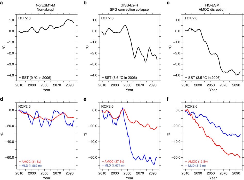
Figure 1. Example of General Circulation Model (GCM) outcomes that expose disagreement among models.

This is demonstrated in Figure 1, which shows change in subpolar gyre sea surface temperature (SST) in degrees Celsius (top row), relative change in AMOC transport (in bottom row, red) and subpolar gyre mixed layer depth (bottom row, blue) in three classes of models used in CMIP5 model intercomparison project. The left column model has a steady rise in temperatures and relatively small decline in overturning. The middle column shows a convective shutoff within the subpolar gyre, though with a relatively weak impact on the overturning. The right column shows a model with a more gradual state transition in temperature, mixed layer depth and overturning.  (Sgubin et al., 2017)

Additionally, as illustrated above in Figure 1 (Sgubin et al., 2017), some models show a shutoff in convection in the Labrador Sea (illustrated by a relatively large relative decline in mixed layer depth and cooling of the subpolar gyre in the models in the center and right-hand columns). These are sometimes accompanied by large relative declines in the overturning circulation while other (illustrated by the model in the left-hand column) models do not. The source of these differences is not well understood across GCMs. One reason for this is that these models differ in many ways, ranging from the numerical techniques used to discretize the Navier-Stokes equations to the representation of ocean mixing to the temperature dependence of sea ice albedo to the response of clouds to changes in stratification. The other reason is that internal model variability may play a role in setting the exact timing of such rapid changes.

AMOC Collapse

Theories for AMOC collapse dating from Stommel (1961) have focused on the role of the enhanced hydrological cycle in driving a hypothesized fold bifurcation. The dynamics of this bifurcation involve greater freshwater flux to the subpolar gyre, increasing the salinity difference and lowering the density difference between high and low latitudes. The result is a slowing of the overturning, which in turn allows more freshwater to build up in high latitudes. Within the Stommel theory, one can define a solution for the mean state overturnings that depends on the overturning driven by temperature alone (\(M_{T}\)), the density difference associated with temperature (\(\Delta\rho_{T}\)), and the maximum density difference associated with salinity (\(\Delta\rho_{S}^{\max}\)) such that the relationship between the overturning and the freshwater flux is:

\[F_{w}\ = \left( \frac{\Delta\rho_{T}}{\Delta\rho_{S}^{\max}}\ \right)*M*\left( M_{T} - M \right)\]

There is then a separatrix that separates the solution state space into regions of stable and unstable solutions defined by:

\[F_{w}\ = \left( \frac{\Delta\rho_{T}}{\Delta\rho_{S}^{\max}}\ \right)*\frac{M_{T}^{2}}{2}\]

This model would then suggest that models that have a larger overturning should be more resistant to collapse. However, this appears to fail in Fig. 1, as the steepest drop in temperature is found in the model with intermediate overturning. Nor does the initial depth of convection in the Labrador Sea appear to explain the difference (both the left-hand and middle column appear to have realistically deep convection).

More recent theories note that there are multiple controls on the overturning, which can be combined in different ways to produce “realistic”-looking results. However, as described in Gnanadesikan et al. (2018), these combinations may have quite different stability thresholds.  A potentially important question is how are salinity anomalies in the upper subpolar gyre removed- is the overturning the dominant mode of removal or is lateral exchange? A second possibility is that the differences reflect different levels of remote forcing from winds in the Southern Ocean, which are expected to increase under global warming and thus to provide a stronger source of light water-stabilizing the overturning. A third possibility is that some models have unrealistic convection in the Northwest Pacific. Under global warming, this convection switches off and the pycnocline as a whole deepens, driving more light water into the North Atlantic and counteracting the “braking” effect from the enhanced hydrological cycle.

Questions to Answer Using Machine Learning

Distinguishing between these multiple controls on the overturning has not been straightforward, suggesting that the application of machine learning methods might be fruitful. In particular, we would like answers to the questions noted below:

1. Do models that exhibit rapid change in AMOC/convection under relatively weak greenhouse gas forcing share some common characteristics in their mean state? Alternatively, do these models have mean states that lies close to the separatrix between “on” and “off” states and what model parameters control the geometry of this separatrix?

2. Do models that exhibit rapid change in AMOC/convection under relatively weak greenhouse gas forcing share some common characteristics in the dynamics of their variability? Another way of stating this would be- do such models have a mean state that is comparably far from the separatrix between “on” and “off” states, but larger internal variability compared with models that don’t show rapid change?

3. Can we predict the magnitude and timing of rapid transitions in AMOC/convection using the behavior of the model in preindustrial control simulations?

4. Do models that show collapse under relatively weak forcing exhibit fingerprints of change that provide early warning?

5. Can we express all of these in terms of a parsimonious representation of the overturning (i.e., neuro-symbolic/box model)?

In some cases, the answers to these questions might reflect systemic model biases. For example, it might be the case that models that have an Icelandic low that is too far to the east will be inefficient at laterally exporting freshwater from the Atlantic and thus more likely to see a collapse. This would lead us to be less concerned about rapid transitions occurring in the next 20-40 years.  Or in another instance, it might be that models that do not show too much sensitivity to global warming have unrealistic convection in the Northwest Pacific-leading us to be more concerned about the possibility of AMOC collapse. Additionally, it is possible that a rapid transition in the AMOC is driven by a particular combination of atmospheric and oceanic conditions that may randomly occur in some models but not others.

Risks/Concerns

A few instances of concern are: a) the real world might lie close to a separatrix, but we haven’t yet experienced the particular combination of conditions that would result in a tipping point and b) inaccuracies in the current generation of models make it impossible to capture this state of affairs. Our goals are to develop an AI system that can explore a set of models, identify models with realistic solutions that lie close to a tipping point, and apply this system to some subset of the CMIP6 models to either generate initial conditions that would produce an early transition of the overturning or identify biases that make such a transition less likely than would be the case in the real world.

4      Task 2.1. CMIPS and PMIP Data Acquisition and Analysis

Description: Acquire CMIPs data and perform a cross-disciplinary analysis of data extractions to formulate the AI datasets to enable the use case.

In order to address the questions laid out above, we will use data from existing global general circulation models (GCM) in concert with the Gnanadesikan et al. (2018) box model as a framework for reducing the data for initial understanding. This model connects the overturning rate to the pycnocline depth at lower latitudes, freshwater fluxes between high and low latitudes, the low-latitude upwelling from depth, and the Southern ocean’s balance of wind-driven and eddy-driven fluxes. These state variables can be integrated from the available standard outputs archived for the coupled model intercomparison projects (CMIP) and analyzed for their dynamics in the same way as the box model.

Our initial analysis of the available runs of CMIPs models, with respect to having sufficient representation of AMOC tipping point conditions, has led us to consider a secondary set of model runs – the PMIP4, Paleoclimate Model Intercomparison Project 4 (https://pmip4.lsce.ipsl.fr/doku.php/index), which includes many of the same models as CMIP. The scenarios run in PMIP4 are good candidates for complementing the pre-industrial control runs and forward scenarios from CMIP.

Using the Community Earth System Model

We will begin with the Community Earth System Model (CESM), as we know that there are significant changes in the North Atlantic convection for the lower-warming projections of the 21st century (https://doi.org/10.1111/nyas.14659). A large ensemble of pre-industrial control simulations with initializations spanning a range of AMOC strengths (LENS2, CESM2 Large Ensemble Community Project (ucar.edu)) will be used to map out the stable areas in dynamical state space. These simulations include a large number of oscillations in the strength of the AMOC, without reaching a collapse or permanent change in state (see Figure 2 below).  Analyzing the dynamics of this ensemble will allow us to improve the box model, if needed, to have similar stable-AMOC dynamics. The 21st-century projections, on the other hand, may contain a tipping point, which we can determine after the pre-industrial analysis. If these are insufficient to represent the alternate AMOC state, we will also use available paleoclimate runs for this model (Holocene, Pliocene, and Last Interglacial). The paleoclimate simulations have large variations in CO₂ and AMOC, but other forcing changes that are less similar to those expected in the near future. While we will describe it in more detail in the next section, the aim is to understand the dynamics through identifying the separatrix between ‘normal’ subpolar convection and AMOC and a shut-off of subpolar convection and weakened or collapsed AMOC.

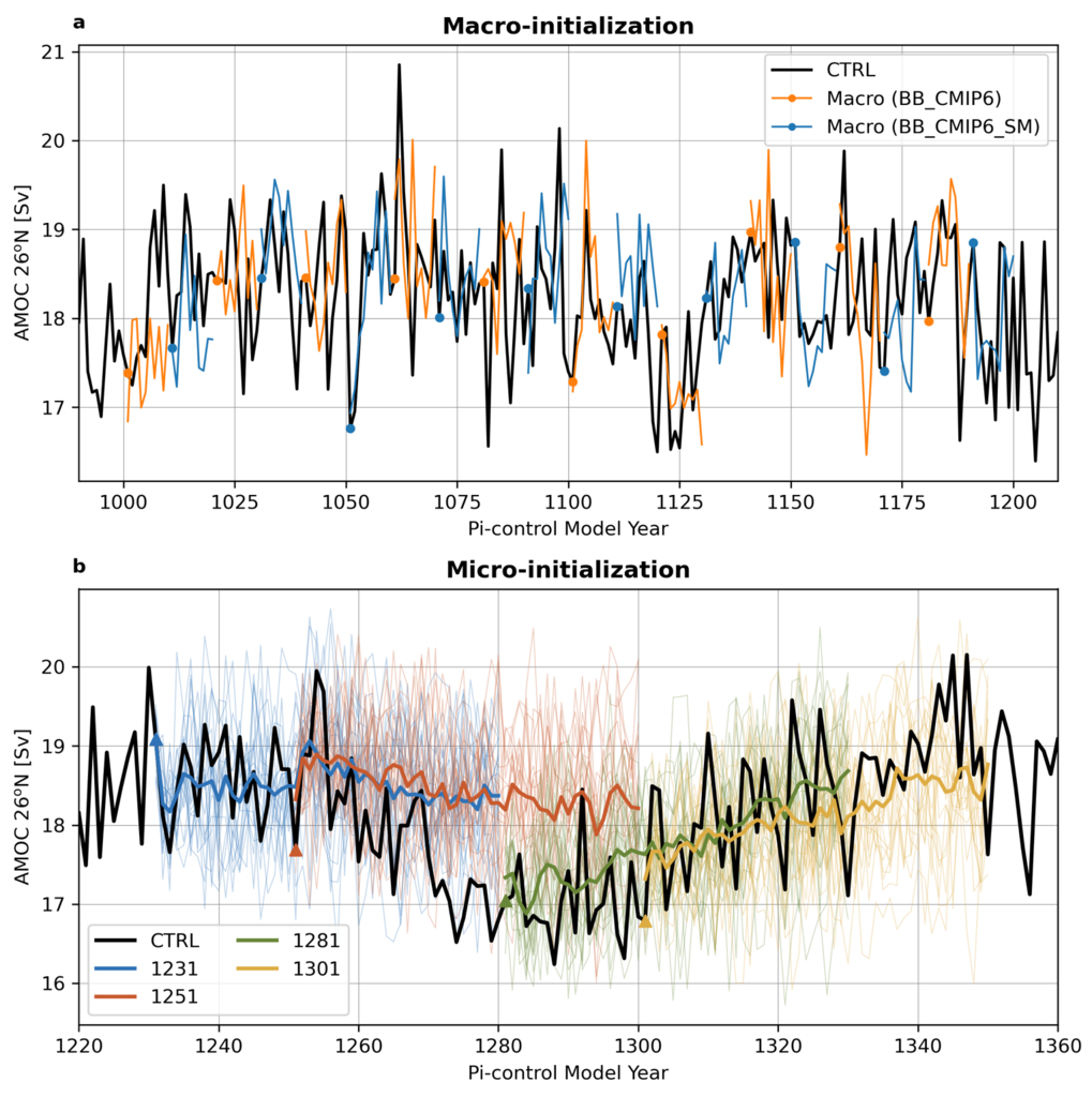
Figure 2. CESM2-LE initialization consequences for the Atlantic Meridional Overturning Circulation (AMOC) at 26.5°N with 20 macro-initializations (top) and the micro-initializations (bottom).

As shown in Figure 2 above, the AMOC transport in the pre-industrial control simulation (black line) for CESM2 is shown over two time slices corresponding to (top) 20 macro-initializations and (bottom) the micro-initializations. In the top figure the AMOC transports for the individual ensemble members are shown as solid colors, with the initiation points marked as colored closed circles. In bottom figure the AMOC transports are shown in thin solid lines for individual ensemble members, and the ensemble-mean is represented as a thicker solid line. Transports are in Sverdrups (Sv) (106 m3 s-1). (Rodgers et. al 2021, https://doi.org/10.5194/esd-12-1393-2021).

The CESM2 Large Ensemble is available through the NCAR Climate Data Gateway (Dataset: CESM2 LENS Ocean Post Processed Data Monthly Averages (earthsystemgrid.org)). The CMIP6 model outputs are available through the CMIP6 portal, https://esgf-node.llnl.gov/search/cmip6. The initial use model has a small ensemble of historical and pre-industrial control (piControl) runs labeled CMIP.NCAR.CESM2; the forward projection with a known strong decrease in subpolar convection is ScenarioMIP.NCAR.CESM2.ssp126 (3 instances). The variables needed to perform this analysis include the wind stress, temperature, salinity, surface heat and water fluxes, and internal mass and freshwater fluxes. We are using the monthly-mean ocean and atmospheric data for this stage. While we are currently reducing the data by integrating across large sections of the Atlantic and Southern Ocean, we expect to use the full data later for the Generative Adversarial Network (GAN). The integrated data may be of interest to the Exeter group, as they examine abrupt changes and possible early warning signals. We plan to share the data and the method for building it so that others can use it across more models.

While we are beginning with a single GCM, as noted in the previous section, our interests, include the differences between models. Thus, once this model whose behavior includes convection collapses is analyzed, we will be able to apply the same techniques to a broader set of CMIP6 GCMs.

Data Storage, Preprocessing and Data Analysis First Steps

We currently have a team performing system requirement analysis for data storage to host this data. The options we are evaluating include: SciServer, Amazon cloud, and an internal high-performance environment. As part of this effort, we are evaluating resource needs based on an initial analysis of the models we will use both with respect to the box model and with respect to the GCMs. Currently, we are serially downloading individual ensemble members and processing them to reach box-model-style integrated timeseries for our initial analyses. We also building a suite of data processing tools to ready the data for machine learning processing. Our cross-disciplinary team is working together in weekly meetings to develop this data repository. Analysis of this data from the machine learning perspective will begin once the data repository is populated with the model data.

Initial discussions have included mapping variables that will be used from the Box models to variables that will be used from the GCMs. Part of this discussion has been to define a set of variables that will be important to include in the model data for deep learning models. As part of this step, we have begun to download example, simplified CESM2 models to perform data analysis.

5      Task 3.1 AI Physics-Informed Surrogate Model Design

Description: Identify the architectures and equations that will be modeled in terms the neural network.

Due to the complexity of GCMs, we are taking the approach of building AI architectures that use simplified box models initially then once the architectures are stabilized progress to the more complex GCMs. The AI simulation is agnostic in that it can work with any type of surrogate model. We list surrogate models and their levels of complexity below (we will start with the zero-dimensional box models and progress to the three-dimensional GCMs):

Types of Surrogate models (increasing in level of complexity):

• Zero-dimensional Ocean models (box models), uses 10 ODEs

• One-dimensional ocean models using PDEs for vertical structure

• Two-dimensional PDE Ocean models

• Three-dimensional General circulation models

As a first pass at developing the surrogate models, we will use the box models as described in Tasks 1.1 and 2.1.

Tipping Point Identification

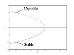
As a basis for tipping point identification, saddle-node (fold) bifurcation identification as shown in Figure 3, will be used to identify sudden changes in the model. Initially, the saddle-node bifurcation method will be applied using both zero-dimension and one-dimension models.

Further extensions to this method will be developed as we begin to work with GCMs. Thus far, our progress in terms of tipping point identification has been to identify tipping points (i.e., saddle-node bifurcations) using the box model as a tool for identifying forcing conditions that result in bifurcation.

We are developing the methodology to perform parametric bifurcation analysis for the Gnanadesikan et al. (2018) box models using established numerical bifurcation/continuation algorithms, to discover the locus of “hard” bifurcations (folds, subcritical Hopf) that are known to underpin model tipping points.

We will then attempt the computation of the slow stable manifolds of the saddle solutions that defines the separatrix (a difficult problem) since in a system with n degrees of freedom the separatrix is an n-1 dimensional manifold. We are only interested in the slowest stable directions. These are the data that will be used to train our GAN surrogate separatrix construction. We are also exploring how to inform/match the box models with “box-level” observations of the finer, PDE Ocean models in the neighborhood of the tipping points.

6      Task 4.1 AI Simulation Design

Description: Evaluate potential architectures, explore the theoretical setup of tipping point identification and identify the requirements of the neuro-symbolic and causal models. We will map how these subsystems will work together as one cohesive framework.

Generative Learning - Overview

The GAN will take the form based on the typical setup of the adversarial game (based on minimax game theory and Nash equilibrium) and Goodfellow 2014, as shown below, where G represents the generator neural network and D represents the discriminator neural network, \(\mathbb{E}_{x}\) represents the expected value over data samples and \(\mathbb{E}_{z}\) represents the expected value over generated samples, with adjusted D parameters to minimize log D(x) and adjusted G parameters to minimize log(1-D(G(x))) define the minimax game. In this adversarial setup, the discriminator tries to maximize its loss and the generator tries to minimize its loss as depicted in the following value function, where V is the value function.

\[\frac{\min}{G}\frac{\max}{D}V(D,\ G) = \ \mathbb{E}_{x\sim pdata(x)}\lbrack\log{D(x)\rbrack + \ }\mathbb{E}_{z\sim p_{z}(Z)}\left\lbrack \log\left( 1 - D\left( G(z) \right) \right) \right\rbrack\]

Labeled data is processed by the discriminator and “fake” data is generated by the generator. The generator distribution is learned by a mapping function that maps from a prior noise distribution pz(z) to the data space.

In the proposed GAN architecture, there will be prior information that constrains the pz(z) distribution, as this will be prescribed symbolically in terms of the problem setup. Therefore, the loss function will need to be modified to account for multiple generators and a single discriminator in addition to having priors. There will be M generators so as G1:M will map to a single distribution representing the perturbations of the model (akin to an ensemble). As each G has access to the model that it perturbed, this goes beyond a mixture over the M distributions because their perturbations are based on a previous step in the adversarial game.

Generative Learning – Surrogate Interaction

In GAN architectures typically a discriminator learns a classification, for example classifying images, and is given labeled information which it uses to determine how well it is learning that classification. In our proposed architecture, the job of the discriminator involves the extension of a surrogate model and bifurcation method that the discriminator uses to run the conditioned scenario. The discriminator uses the surrogate and bifurcation method to classify the conditions presented, as a tipping point or not, and at the same time calculates a loss on its own model based on assessing how imbalanced or balanced the state is, given the presented conditions.

The architecture for the discriminator based on this interaction is still being explored by our team, as we are developing a probabilistic model to support this interaction. Our team is currently working on a simple GAN prototype to understand requirements of the architecture and loss function given this setup. We will first begin with a pure simulated-data prototype, then introduce a simple problem which includes a set of conditions, a simplistic surrogate model, and the 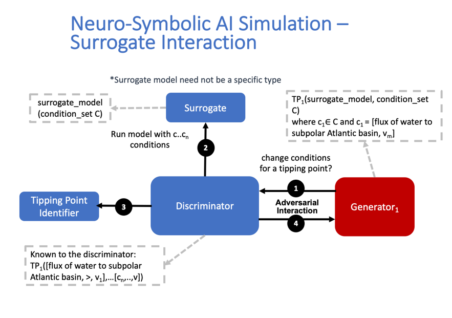bifurcation algorithm. As shown in Figure 4, this part of the exploration is focused on the interactions between the discriminator, a surrogate and a method that tells the discriminator if the identification of a tipping point was reached or not.

The adversarial game is based on this idea climate forcings: where the discriminator’s goal is to keep the forcings balanced, the generators will perturb conditions to unbalance the forcings, defined in terms of positive and negative forcings:

Positive forcings:

• Warming of low latitudes

• Cooling of high latitudes

• Upwelling in subpolar gyre (+North Atlantic Oscillation (NAO)/Arctic

  Oscillation (AO))

• Lateral mixing of salinity by eddies into the mixed layer

• Stronger winds driving more evaporation

Negative forcings:

• Hydrological cycle, salinities tropics and freshens high latitudes

• Loss of glacial land ice (e.g., Greenland Ice Sheet) freshens

  subpolar North Atlantic.

• Warming of high latitudes

• Weak downwelling in subpolar gyre (-NAO/AO?)

• Lateral advection by eddies

• Weaker winds driving less evaporation

The AI simulation is agnostic in that it can work with any type of surrogate model.  As mentioned in Tasks 1.1 and 2.1, given the box model is able to succeed in matching expected behavior at it relates to the separatrix between ‘normal’ convection and a shut-off of convection, a map of the separatrix of the box model will be used by the discriminator for the GAN.  The box model will be introduced in these early experiments as the prototype the AI simulation progresses.  As part of this step forcing imbalances will be identified a priori using the pre-industrial control simulations and historical (years) data (see section 4 for more of a discussion of this data) and a map of the separatrix.

In this early stage, we will not introduce the full neuro-symbolic language for training, but will use a pseudo-representation of this language.

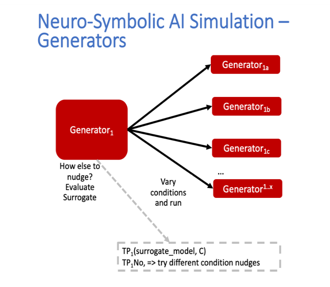
Generative Learning – Generators

The introduction of multiple generators also diverges from a typical GAN architecture, pictured in Figure 5. In work by Hoang et al. 2018 and Li et al. 2021, a multi-generator GAN was introduced to overcome mode collapse issues and to improve performance, however in both of these publications they treated the generators as a mixture over the distributions and used a classifier to perform a multi-class classification associating labels with generators.

We will explore if the classifier is required for the proposed GAN, as we introduced an underlying causal model to capture the state of the model as the generators perturb conditions. To better understand this interaction, the team is working on a prototype that captures state changes across a surrogate model by means of a causal graph structure.

We will be exploring the behavior of this interaction and using that exploration to inform how to constrain the interactions across generators, and how the interaction between the generators and the causal model will take place. In addition, we are considering causality in terms of template causal graph of known knowledge. We will explore how that can be used to constrain the generators’ perturbations so as to ensure the generators are not going down paths in the model space that are unrealistic.

Neuro-symbolic Language Requirements

The team has begun to identify requirements for the neuro-symbolic language.  This language will be critical for symbolically representing questions formulated that will be asked of the model and will define the parameters for adversarial game.

A requirement for the neuro-symbolic language is that we bound the language to a small enough subset that the representation is maintainable, but large enough to capture the scenarios that lead to forcing imbalances.

The language will include the following representations:

Ocean regions (and potential sub-regions):

• Arctic

• Atlantic (North Atlantic)

• Indian

• Pacific (North Pacific)

• Southern oceans

• Tropics

• Equatorial band

• High and Low Latitudes

• Surface

• Deep

• Subsurface

In addition, equatorial, subtropical, and subpolar separations of the Arctic, Atlantic, Pacific, Indian ocean may be useful sub-regions.

The following categories of parameters (with specific parameters defined for each category):

• Air (Temperature)

• Wind (Speed, Direction)

• Water (Temperature, Salinity, Density)

• Current (Direction, Flow, Velocity, Integrated overturning flux in depth and density space)

• Sea Surface (Height, Temperature)

Our team is also working on defining the symbolic representation of the problem setup-ups that will be used for the adversarial interactions. This includes symbolically representing:

• Questions to enable the GAN exploration

• Model initial conditions

• Conditions

• Bounds in terms of conditions

• Tipping Point Probability thresholds

For GAN simulation, there will be a set of parameters which constrain and direct the adversarial game and a set of parameters that act as hyperparameters for the GAN itself. We will further define these parameters as we move forward with prototyping the architectures.

Causality

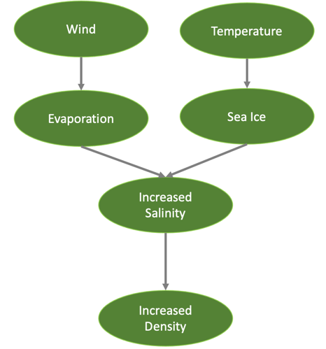There are two ways in which causality will be used to support the AI Simulation.  The first we are evaluating is using causal structure “templates” as part of the symbolic representation of the problem domain.  For example, as shown in Figure 6, we know generally that evaporation leads to high salinity in ocean waters, and that sea ice can also lead to higher levels of salinity. An increase in salinity can lead to an increase in density which could then have other effects. However, what we wish to learn are the co-occurring factors and the probabilistic model that governs these co-occurring factors. Our team is currently defining these potential causal structure “templates” and evaluating how these templates will be used. As we build the neuro-symbolic language, this kind of causal structure can help structure how the generators build out graph structures which support their search in parameter space.

The second area where causality will be implemented is as a post-processing inference applied to the causal graph constructed as a result of the adversarial game played between the generators and the discriminator.  We are currently developing a causal inference method that will use the adversarial generated graph structure to infer the following: a) subspaces that the climate model should explore to invoke a tipping point (directed search), b) an explainability map to better characterize the adversarial game, and c) to support question answering of the graph. We are exploring a graphical model and a machine learning method for this work.

Conclusion and Next Steps

The first milestone marks a concentrated effort to clearly define how we will model and invoke abrupt state changes in the AMOC, which models will be used to formulate datasets, initial prototype definitions for the AI models, and a plan for setting up the computing environment to enable joint research between the APL and JHU teams. Part of this effort has been to think through risks both in terms of computational needs and in terms of collecting the right data to sufficiently support deep learning research, in particular producing sufficient examples of AMOC tipping point conditions for training.

The next steps include continuing to perform data analysis on both the box models and the GCM models which will be used to build a AI data repository, to run simulations using the box model to generate tipping model conditions, to begin building prototype deep learning architectures and to further define the function of these architectures, to develop the first version of neuro-symbolic language and its role with the underlying causality model, and to build the first version of surrogate models and accompanying bifurcation method.

Bibliography

Gnanadesikan, A., R. Kelson and M. Sten, Flux correction and overturning stability: Insights from a dynamical box model, J. Climate, 31, 9335-9350, https://doi.org/10.1175/JCLI-D-18-0388.1, (2018).

Stommel, H. Thermohaline convection with two stable regimes of flow. Tellus 13, 224–230 (1961).

Sgubin, Giovanni, Didier Swingedouw, Sybren Drijfhout, Yannick Mary, and Amine Bennabi. “Abrupt cooling over the North Atlantic in modern climate models.” Nature Communications 8, no. 1 (2017): 1-12.

Rodgers, Keith B., Sun-Seon Lee, Nan Rosenbloom, Axel Timmermann, Gokhan Danabasoglu, Clara Deser, Jim Edwards et al. “Ubiquity of human-induced changes in climate variability.” Earth System Dynamics 12, no. 4 (2021): 1393-1411.

Goodfellow, Ian, Jean Pouget-Abadie, Mehdi Mirza, Bing Xu, David Warde-Farley, Sherjil Ozair, Aaron Courville, and Yoshua Bengio. “Generative adversarial nets.” Advances in neural information processing systems 27 (2014).

Hoang, Quan, Tu Dinh Nguyen, Trung Le, and Dinh Phung. “MGAN: Training generative adversarial nets with multiple generators.” In International conference on learning representations. 2018.

Li, Wei, Zhixuan Liang, Julian Neuman, Jinlin Chen, and Xiaohui Cui. “Multi-generator GAN learning disconnected manifolds with mutual information.” Knowledge-Based Systems 212 (2021): 106513.